Test Driven Development on an SQL Database Schema

TDD on SQL Schema. Why not? A normal Test Driven Development approach means that you start with writing a test case which creates the requirement to write appropriate code in order for the test to pass. This results in a very quick iteration where you add new unit tests, verify that they fail, implement the code for the test to pass and verify that the test passes. A single iteration can be just few minutes or less and the test set usually executes in just a few seconds. The end result is that you will end up with great test coverage which helps refactoring and in itself it helps explaining the user stories in the code.

Applying TDD to SQL

At first writing CREATE TABLE declarations doesn’t sound like something worth testing, but modern SQL database engines offer a lot of tools to enforce proper and fully valid data. Constraints, foreign keys, checks and triggers are commonly used to validate that invalid or meaningless data is not stored in the database. This means that you can certainly write a simple CREATE TABLE declaration and run with it, but if you want to verify that you cannot send invalid data to a table then you need to test for it. If you end up writing triggers and stored procedures it is even more important to write proper tests.

I picked up Ruby with it’s excellent rspec testing tool for a proof-of-concept implementation for testing a new schema containing around a dozen tables and stored procedures. Ruby has a well working PostgreSQL driver and writing unit test cases with rspec is efficient in term of lines of code. Also as Ruby is interpreted executing a unit test suite is really fast. In my case a set of 40 test cases takes less than half a second to execute.

Example

Take this simple twitter example. I placed a complete source code example in github at https://github.com/garo/sql-tdd

CREATE TABLE users (
    id SERIAL PRIMARY KEY,
    login VARCHAR(20) NOT NULL UNIQUE,
    full_name VARCHAR(40) NOT NULL
);

CREATE TABLE tweets (
    id SERIAL PRIMARY KEY,
    user_id INTEGER REFERENCES users(id) NOT NULL,
    tweet VARCHAR(140) NOT NULL
);

The test suite will first drop the previous database, import the schema into the database from schema.sql following with any optional and non-essential data from data.sql and then run the each unit test case. Our first test might be to verify that the tables exists:

it "has required tables" do
  rs = @all_conn.exec "SELECT table_name FROM information_schema.tables WHERE table_schema = 'public'"
  tables = rs.values.flatten
  expect(tables.include?("users")).to eq(true)
  expect(tables.include?("tweets")).to eq(true)
end

Maybe test that we can insert users into the database?

it "can have user entries" do
  ret = @all_conn.exec "INSERT INTO users(login, full_name) VALUES('unique-user', 'first') RETURNING id"
  expect(ret[0]["id"].to_i).to be > 0

  ret = @all_conn.exec "SELECT * FROM users WHERE id = #{ret[0]["id"]}"
  expect(ret[0]["login"]).to eq("unique-user")
  expect(ret[0]["full_name"]).to eq("first")
end

Verify that we can’t insert duplicated login names:

it "requires login names to be unique" do
  expect {
    ret = @all_conn.exec "INSERT INTO users(login, full_name) VALUES('unique-user', 'second') RETURNING id"
  }.to raise_error(PG::UniqueViolation)
end

What about tweets? They need to belong to a user, so we want to have a foreign key. Especially we want that you can’t violate the foreign key constraint:

describe "tweets" do
  it "has foreign key on user_id to users(id)" do
    expect { # the database doesn't have a user with id=0
      ret = @all_conn.exec "INSERT INTO tweets(user_id, tweet) VALUES(0, 'test')"
    }.to raise_error(PG::ForeignKeyViolation)
  end
end

If you want to test for a trigger validation using a stored procedure then that violation would raise a PG::RaiseException. Using invalid value for an ENUM field would raise a PG::InvalidTextRepresentation. You can also easily test views, DEFAULT values, CASCADE updates and deletes on foreign keys and even user privileges. Happy developing!

Having Fun With IoT

With the blazing fast technology progress it’s now easier than ever to build all kinds of interconnected gadgets, something which the corporate world might refer as IoT – Internet Of Things. For me, it’s just an excuse to spend time playing around with electronics. I’ve been installing all kinds of features into our summer cottage (or mökki, as it’s called in Finnish), so this blog post shows around some things which I’ve done.

All the things where Raspberry Pi is useful!

I’ve lost count how many Raspberry Pi’s I’ve installed. Our cottage has two of them. My home has couple. My office has at least 20 of them. My dog would probably carry one as well, but that’s another story. As Pi runs standard Linux, all the standard Linux knowledge applies, so we can run databases, GUI applications and do things with your favourite programming language.

So far I’ve found it useful to do:

  • Connect our ground heating pump (maalämpöpumppu) to a Raspberry Pi with a usb-serial cable. This gives me full telemetry and remote configuration capabilities, allowing me to save energy by keeping the cottage temperature down when I’m not there and to warm it up before I arrive.
  • Work as a wifi-to-3g bridge. With a simple USB-3G dongle, an USB-WIFI dongle and a bit of standard Linux scripts you can have it to work as an access point for the Internet.
  • Display dashboards. Just hook the Pi up into a TV with HDMI, run Chrome or Firefox in full screen mode and let it display whatever information best floats your boat.
  • Connect DS18b20 temperature sensors. These are the legendary tiny Dallas 1-wire sensors. They look like transistors, but instead they offer digital temperature measurements from -55’C to +125’C in up to 0.5’C resolution. I have several them around, including in Sauna and in the lake. You can buy them in pre-packaged into the end of a wire or you can solder one directly to your board.
  • Run full blown home automation with Home Assistant and hook it up into a wireless Z-Wave network to control your pluggable lighting, in-wall installed light switches or heating.

All the things where a Raspberry Pi is too big

Enter Arduino and ESP8266. Since its introduction in 2005, the Arduino embedded programming ecosystem has revolutionized DIY electronics, opening the doors to build all kinds of embedded hobby systems easily. Recently a Chinese company built a chip containing full Wifi and TCP/IP stack, perfectly suitable to be paired with Arduino. So today you can buy a full WiFi capable Arduino chip (NodeMCU) for less than three euros a piece. With a bit care you can build remote sensors capable of operating under battery power for an impressive amount of time.

Using Raspberry Pi to log temperatures

The DS18b20 sensors are great. They can operate with just two wires, but it’s best to use a three wire cable: One is for ground, another is for operating power and 3rd is for data. You can put them comfortably over 30 meters away from the master (your raspberry pi) and you can have dozens of sensors in a same network as they each have a unique identifier. Reading temperature values from them is also easy as most Raspberry Pi distributions have easy-to-use drivers for them by default. The sensors are attached to the Raspberry Pi extension bus with a simple pull-down resistor. See this blog post for more info. Here’s my code to read sensor values and write the results into MQTT topics.

Using MQTT public-subscribe messaging for connecting everything together.

MQTT is a simple public-subscribe messaging system widely used for IoT applications. In this example we publish the read sensor values to different MQTT topics (for example I have nest/sauna/sauna for the temperature of sauna. I just invented that every topic in my cottage begins with “nest/”, then the “nest/sauna” means values read by the raspberry pi in the sauna building and then the last part is the sensor name).

On the other end you can have programs and devices reading values from an MQTT broker and reacting based on those values. The usual model is that each sensor publishes their current value to the MQTT bus when the value is read. If the MQTT server is down, or a device listening for the value is down, then the value is simply lost and the situation is expected to be recovered when the devices are back up. If you care for getting a complete history even during downtime, you need to build some kind of acknowledgment model, which is beyond the scope of this article.

To do this you can use mosquitto which can be installed into a recent Raspbian distribution with simply “apt-get install mosquitto”. The mosquitto_sub and mosquitto_pub programs are in the “mosquitto-clients” package.

Building a WiFi connected LCD display

My latest project was to build a simple wifi connected LCD display to show the temperature of the Sauna and the nearby lake, and emit a buzzer beep when one needs to go and put more wood in the fireplace when the sauna is warming up.

Here’s the quick part list for the display. You can get all these from Aliexpress for around 10 euros total (be sure to filter for free shipping):

  • A NodeMCU ESP8266 Arduino board from Aliexpress.
  • An LCD module. I bought both 4*20 (Google for LCD 2004) and 2*16 (LCD 1602), but the boxes I ordered were big enough only for the smaller display.
  • An I2C driver module for the LCD (Google for IIC/I2C / Interface LCD 1602 2004 LCD). This is used to make connecting the display to Arduino a lot easier.
  • Standard USB power source and a micro-usb cable.
  • A 3.3V buzzer for making the thing beep when needed.
  • A resistor to limit the current for the buzzer. The value is around 200 – 800 Ohm depending on the volume you want.

Soldering the parts together is easy. The I2C module is soldered directly to the LCD board and then four wires are used to connect the LCD to the NodeMCU board. The buzzer module is connected in series with the resistor between a ground pin and a GPIO pin on the NodeMCU (this is needed to limit the current used by the buzzer. Otherwise this would fry the Arduino GPIO pin). The firmware I made is available here. Instructions on how to configure Arduino for the NodeMCU are here.

When do I need to add more wood to the stove?

One you have your sensors measuring things and devices capable acting on those measurements, you can build intelligent logic to react on different situations. In my case I wanted to have my LCD device to buzz when I need to go outside to add more wood to the sauna’s stove when I’m heating the sauna. Handling this needs some state to track the temperature history and to execute some logic to determine when to buzz. All this could be programmed into the Arduino micro-controller running the display, but modifying this requires to reprogram the device by attaching a laptop with USB to the device.

I instead opted into another way: I programmed my LCD to be stupid. It simply listens MQTT topics for orders what to display and when to buzz. Then I placed a ruby program in my raspberry pi which listens for the incoming measurements about the sauna temperature and where all the business logic is handled. Then this script will order the LCD to display current temperature, or any other message for that matter (for example the “Please add more wood” message). The source code for this is available here.

The program listens for the temperature measurements and stores them in a small ring buffer. Then on each received measurement it calculates the temperature change in the last five minutes. If the sauna is heating up and the change in the last 5min is less than two ‘C warmer, then we know that the wood is almost burned up and we need to signal the LCD to buzz. The program also has a simple state machine to determine when to do the tracking and when it needs to be quiet. The same program also formats the messages which the LCD displays.

Conclusions

You can easily build intelligent and low-cost sensors to measure pretty much any imaginable metric in a modern environment. Aliexpress is full of modules for measuring temperature, humidity, CO2 levels, flammable gases, distance, weight, magnetic fields, light, motion, vibrations and so on. Hooking them together is easy using either Raspberry Pi or an ESP8266/Arduino and you can use pretty much any language to make them act together intelligently.

Any individual part here should be simple to build and there are a lot of other blog posts, tutorials and guides all around the net (I tried to link some of them in this article). Programming an Arduino is not hard and the ecosystem has very good library for attaching all kinds of sensors into the platform. Managing a Raspberry Pi is just like managing any other Linux. When you know that things can be done then you just need some patience while you learn the details and make things work as you want.

Problems with Terraform due to the restrictive HCL.

Terraform is a great tool to define cloud environments, virtual machines and other resources, but sadly it’s default usage of HCL (Hashicorp Configuration Language) is very restrictive and makes IaaC (Infrastructure-as-a-code) look more like Infrastructure-as-copy-paste. Here are my findings on all different issues which makes writing Terraform .tf files with HCL pain (as on Terraform v0.7.2). This is usually fine for most simple scenarios, but if you think like a programmer you will find HCL really restrictive when you encounter any of its limitations.

Make no mistake: Nothing said here are showstoppers, but they simply make you write more code than what would be required and you will also need to repeat yourself a lot by doing copy-paste and that’s always a recipe for errors.

Template evaluation.

Template evaluation with template_file. Variables must all be primitives. So you can’t pass a list to a template and then use that list to iterate when rendering a template. Also you can’t use any control structures inside a template. You can still use all built-in functions and you also need to escape the template file if the syntax collides with the Terraform template syntax.

Module variables

Modules can’t inherit variables without explicitly declaring them each time a module is used, or there are no global variables a module could access. This leads to the need to pass every possible required variable in every possible moment when a module is called. Consider rather static variables like “domain name”, “region” or the amazon ssh “key_name”. This leads to manual copy-paste repetition. Issue #5480 tries to address this.

Also when you use a module, you will declare a name for it (standard terraform feature). But you can’t access that name as a variable inside that module (#8706).

module "terminal-machine" {
  source = "./some-module"
  hostname = "terminal-machine" # there is no way to avoid writing the "terminal-machine" twice as you can't access the module name.
}

Variables are not really variables

Terraform supports variables which can be used to store data and then later pass that to a resource or a module, or use those to evaluate expressions when defining a module variable. But there are caveats:

  • You can’t have intermediate variables. This for example prevents you for setting a map which values evaluate from variables and then later merge that map with a module input. You can kinda work around with this with a null_resource, but it’s a hack.
  • You can’t use a variable when defining a resource name: “interpolated resource names are considered an anti-pattern and thus won’t be supported.”
  • You can’t evaluate a variable which name contains a variable. So you can’t do something like this “${aws_sns_topic.${topic.$env}.arn}”.
  • If you want to pass a list to a resource variable which requires a list, you need to encapsulate it again into a list: security_groups = [${var.mylist}]. This looks weird to a programmer.

Control structures and iteration

No control structures, iteration nor loops. HCL is just syntactic sugar for JSON. This means that (pretty much) all current features for iteration in Terraform are implemented inside Terraform itself. So you can have a list of items and use that list to spawn a resource which is customised using the list entries using interpolation syntax:

variable "names" {
  type = "map"
  default = {
    "0" = "Garo"
    "1" = "John"
    "2" = "Eve"
  }
}

resource "aws_instance" "web" {
  count = "${length(var.names)}"

  tags {
    Name = "${element(var.names, count.index)}'s personal instance"
  }
}

This works so that Terraform evaluates the length() function to assign count amount of items there are in the map names and then instantiating the resource aws_instance that many times. Each instantiation evaluates the element() function, so we can customise that instance. This doesn’t however extend to more depth. Say you want that each user has three different instances, one for testing and another for staging. You can’t define another list environments and expect to use both names and environments to declare resources in a nice ways. There are couple of workarounds [1] [2], but they usually really complex and error prone. Also you can’t easily reference a property (such as arn or id) of a created resource in another resource, if the first resource tries to use this kind of interpolation.

A programmers approach would be something like this:

variable "topics" {
  default = ["new_users", "deleted_users"]
}

variable "environments" {
  default = ["prod", "staging", "testing", "development]
}

for $topic in topics {
  # Define SNS topics which are shared between all environments
  resource "aws_sns_topic" "$topic.$env" { ... }

  for $env in environments {
    # Then for each topic define a queue for each env
    resource "aws_sqs_queue" "$topic.$env-processors" { ... }

    # And bind the created queue to its sns topic
    resource "aws_sns_topic_subscription" "$topic.$env-to-$topic.$env-processors" {
      topic_arn = "${aws_sns_topic.${topic.$env}.arn}"
      endpoint = "${aws_sqs_queue.{$topic.$env-processors}.arn}"
    }
  }
}

But that’s just not possible, at least currently. Hashicorp argues that control structures remove the declarative nature of HCL and Terraform, but I would argue that you can still have a language with declarative nature which declares resources and constant variables, but still have control structures like in pure functionally programming languages.

Workarounds?

There have been few projects which have created for example a Ruby DSL which outputs JSON directly into Terraform but they aren’t really maintained. Other options would be to use for example C preprocessor, or just hit a nail into your head and accept that you need to do a lot of copy-pasting and try to minimize the amount of infrastructure which is provisioned using Terraform. It’s still a great tool once you have your .tf files ready: It can query current state, helps with importing existing resources and the dependency graph works well. Hopefully Hashicorp realises that the current HCL could be extended much more while still maintaining its declarative nature.

Cassandra cluster migration story

This is a simple story how we migrated a live production cluster with all its data into a new cluster, all without downtime.

Old cluster:

  • 60 c4.4xlarge instances
  • Cassandra 2.1.12, 256 vnodes per host
  • Each instance had two 1500 GB GP2 EBS disks. This matches the c4.4xlarge EBS bandwidth quite well as max bandwidth for the instance is 250 MB/sec and the max EBS bandwidth is 160 MB/sec per disk.
  • Total of 39 TiB of data with replication factor 3

New cluster:

  • 72 i2.4xlarge instances, ephemeral SSDs
  • Cassandra 2.2.7, no vnodes
  • Initial import resulted in ~95 TiB of data.
  • Initial compaction estimation was 21 days. Total compaction time around one week.
  • 25 TiB of data after compaction.

Migration plan

We did a hot migration which we have done several times in the past. It’s based on the fact that all our operations are impotent in a way that we can do dual writes to both the old and the new cluster from our application. Once the dual writes have started we will know that all data from that point on will be stored on both the old and the new cluster. Then we initiate a BulkLoad operation from the old cluster to the new cluster, where we stream all SSTables into the new cluster instances.

When Cassandra does writes, it will store data with a timestamp field to the disk. When a field is updated a new record is created to a new SSTable which points to the same key, has the new value and most importantly has a newer timestamp. When Cassandra does reads it will read all entries, group them by the keys and then select only the newest entries for each key according to the timestamps.

We can leverage this behavior by BulkLoading all SSTables from the old cluster into the new cluster as any duplicated data will be handled automatically on the Cassandra read code path! In other words, it will not matter if we copy data from the old cluster to the new cluster which has already been written to the new cluster by the application doing dual writes. This fact makes migrations like this really easy and we can do these without any downtime.

So the steps are:

  1. Create new cluster and create keyspaces and table schemas into the new cluster.
  2. Modify application to write both the old and the new clusters. Keep the application reading from the old cluster.
  3. Run BulkLoader in every node in the old cluster so that it will read all SSTables from the instance in the old cluster and feed them into the new cluster.
  4. Wait that Cassandra compacts the loaded data.
  5. Do a incremental repair round so that all current data is incremental repaired once.
  6. Switch the application to do reads from the new cluster.
  7. Disable writes to the old cluster after you are sure that the new cluster works and can hold the load; you could still rollback to the previous cluster until this point.
  8. Destroy the old cluster.

Compaction phase

After the BulkLoader each instance in the new cluster will have a lot of SSTables which need to be compacted. This is especially the case if you streamed from every instance in the old cluster, so you should have three copies of every data (assuming ReplicationFactor 3) on every instance. This is normal, but this will take some time.

Initially each cluster instance had around 7000-8000 pending compactions, so the entire cluster had over half million pending compactions. Once streaming was completed the compaction started right away and in the end it took around one week. At the beginning the compaction speed felt slow: After one days worth of compaction I estimated that at that run rate it would take three weeks to compact everything. During the compaction each instance had one or two moments where only one giant compaction task was running for around one day and this seems normal. After this task was done then the Pending Compactions count dropped by several thousands and the remaining compactions went quite fast. If we look on the OpsCenter the PendingCompactions chart looked something like this in the end.

Because the bootstrap created a lot of small SSTables in L0 the Leveled Compaction switched to using STCS in L0, which resulted in a few big SSTables (from 20-50 GiB in size). This can be avoided by using the stcs_in_l0 flag in the table: ALTER TABLE … WITH compaction = {‘class’:’LeveledCompactionStrategy’, ‘stcs_in_l0’: false}; I did not use this and thus some of my compactions after repairs take longer than they might actually require.

Incremental repairs

We also switched to use Incremental Repairs (they are the new default in 2.2), so we ran couple of full repair cycles on the new cluster while it was still receiving only a partial production load. This gave us valuable information how we should tune streaming throughput and compaction threads in the new cluster to ensure values which don’t affect production. We ended up settling up with five compaction threads (out of 16 CPU cores).

Conclusions

Overall the migration went really well. Assuming you can make a code change which will do dual writes into two different cluster, this method is really nice if you need to migrate a cluster into a completely new one. Reasons for doing this kind of migration could be major revision number, changing deployment topology or perhaps changing machine type. This allows a nice way to rollback at any given moment, greatly reducing operational risks.

Problems With Node.JS Event Loop

Asynchronous programming with Node.JS is easy after getting used to it but the single threaded model on how Node.JS works internally hides some critical issues. This post explains what everybody should understand on how the Node.JS event loop works and what kind of issues it can create, especially on high transactional volume applications.

What The Event Loop Is?

In the central of Node.JS process sits a relatively simple concept: an event loop. It can be thought as a never ending loop which waits for external events to happen and it then dispatches these events to application code by calling different functions which the node.js programmer created. If we think this really simple node.js program:

setTimeout(function printHello () {
    console.log("Hello, World!");
}, 1000);

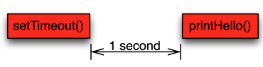
When this program is executed the setTimeout function is called immediately. It will register a timer into the event loop which will fire after one second. After the setTimeout call the program execution freezes: the node.js event loop will patiently wait until one second has elapsed and it then executes the printHello() function, which will print “Hello World!”. After this the event loop notices that there’s nothing else to be done (no events to be scheduled and no I/O operations underway) and it exists the program.

We can draw this sequence like this where time flows from left to right: The red boxes are user programmable functions. In between there’s the one second delay where the event loop sits waiting and until it eventually executes the printHello function.

Let’s have another example: a simple program which does a database lookup:

var redis = require('redis'), client = redis.createClient();
client.get("mykey", function printResponse(err, reply) {
    console.log(reply);
});

If we look closely on what happens during the client.get call:

  1. client.get() is called by programmer
  2. the Redis client constructs a TCP message which asks the Redis server for the requested value.
  3. A TCP packet containing the request is sent to the Redis server. At this point the user program code execution yields and the Node.JS event loop will place a reminder that it needs to wait for the network packet where the Redis server response is.
  4. When the message is receivered from the network stack the event loop will call a function inside the Redis client with the message as the argument
  5. The Redis client does some internal processing and then calls our callback, the printResponse() function.

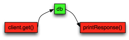
We can draw this sequence on a bit higher level like this: the red boxes are again user code and then the green box is a pending network operation. As the time flows from left to right the image represents the delay where the Node.JS process needs to wait for the database to respond over network.

Handling Concurrent Requests

Now when we have a bit of theory behind us lets discuss a bit more practical example: A simple Node.JS server receiving HTTP requests, doing a simple call to redis and then return the answer from redis to the http client.

var redis = require("redis"), client = redis.createClient();
var http = require('http');

function handler(req, res) {
	redis.get('mykey', function redisReply(err, reply) {
	  res.end("Redis value: " + reply)
	});
}

var server = http.createServer(handler);
server.listen(8080);

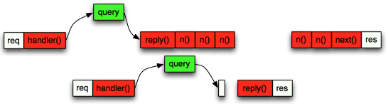
Let’s look again an image displaying this sequence. The white boxes represent incoming HTTP request from a client and the response back to that client.

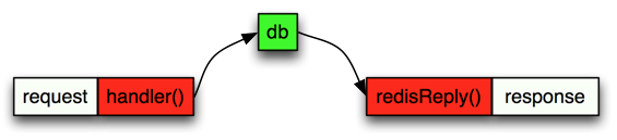
So pretty simple. The event loop receives the incoming http request and it calls the http handler immediately. Later it will also receive the network response from redis and immediately call the redisReply() function. Now lets examine a situation where the server receives little traffic, say a few request every few second:

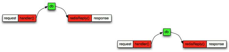
In this sequence diagram we have the first request on “first row” and then the second request later but drawn on “second row” to represent the fact that these are two different http request coming from two different clients. They are both executed by the same Node.JS process and thus inside the same event loop. This is the key thing: Each individual request can be imagined as its own flow of different javascript callbacks executed one after another but they are all actually executing in the same process. Again because Node.JS is single threaded then only one javascript function can be executing simultaneously.

Now The Problems Start To Accumulate

Now as we are familiar with the sequence diagrams and the notation I’ve used to draw how different requests are handled in a single timeline we can start going over different scenarios how the single threaded event loop creates different problems:

What happens if your server gets a lot of requests? Say 1000 requests per second? If each request to the redis server takes 2 milliseconds and as all other processing is minimal (we are just sending the redis reply straight to the client with a simple text message along it) the event loop timeline can look something like this:

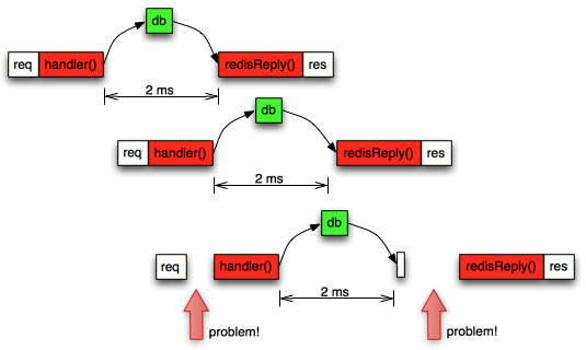
Now you can see that the 3rd request can’t start its handler() function right away because the handler() on the 2nd request was still executing. Later the redis reponse from the 3rd arrived after 2ms to the event loop, but the event loop was still busy executing the redisReply() function from the 2nd request. All this means that the total time from start to finish on the 3rd request will be slower and the overall performance of the server starts to degrade.

To understand the implications we need to measure the duration of each request from start to finish with code like this:

function handler(req, res) {
        var start = new Date().getTime();
	redis.get('mykey', function redisReply(err, reply) {
	  res.end("Redis value: " + reply);
          var end = new Date().getTime();
          console.log(end-start);
	});
}

If we analyse all durations and then calculate how long an average request takes we might get something like 3ms. However an average is a really bad metric because it hides the worst user experience. A percentile is a measure used in statistics indicating the value below which a given percentage of observations in a group of observations fall. For example, the 20th percentile is the value (or score) below which 20 percent of the observations may be found. If we instead calculate median (which means 50%), 95% and 99% percentile values we can get much better understanding:

  • Average: 3ms
  • Median: 2ms
  • 95 percentile: 10ms
  • 99 percentile: 50ms

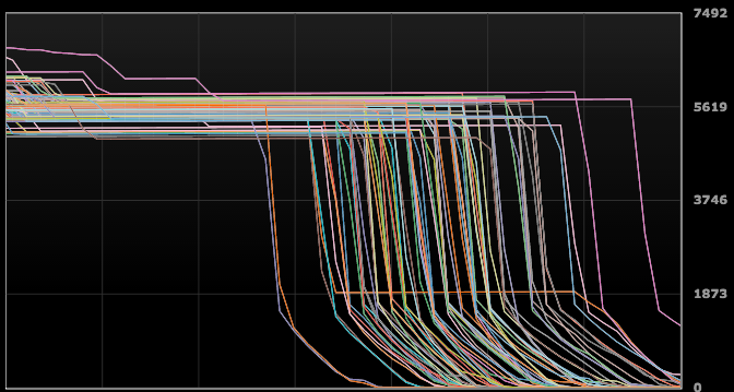
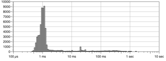
This shows the scary truth much better: for 1% of our users the request latency is 50 milliseconds, 16 times longer than average! If we draw this into graph we can see why this is also called a long tail: On the X-axis we have the latency and on the Y axis we have how many requests were completed in that particular time.

So the more requests per second our server servers, the more probability that a new request arrives before the previous is completed rises and thus the probability that the request is blocked due to other requests increases. In practice, with node.js when the server CPU usage grows over 60% then the 95% and 99% latencies start to increase quickly and thus we are forced to run the servers way below their maximum capacity if we want to keep our SLAs under control.

Problems With Different End Users

Let’s play with another scenario: Your website servers different users. Some users visit the site just few times a month, most visit once per day and then there are a small group of power users, visiting the site several times per hour. Lets say that when you process a request for a single user you need to fetch the history when the user visited your site during the past two weeks. You then iterate over the results to calculate whatever you wanted, so the code might look something like this:

function handleRequest(res, res) {
	db.query("SELECT timestamp, action from HISTORY where uid = ?", [request.uid], function reply(err, res) {
	  for (var i = 0; i < res.length; i++) {
	  	processAction(res[i]);
	  }
	  res.end("...");
	})
}

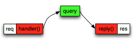
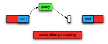
A sequence diagram would look pretty simple:

For the majority of the sites users this works really fast as a average user might visit your site 20 times within the past two weeks. Now what happens a heavy user hits your site which has visited the site 2000 times the past two weeks? The for loop needs to go over 2000 results instead of just a handful and this might take a while:

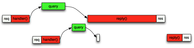
As we can see this immediately causes delays not only to the power user but all other users which had the back luck of browsing the site at the same time when a power user request was underway. We can mitigate this by using process.nextTick to process a few rows at a time and then yield. The code could look something like this:

var rows = ['a', 'b', 'c', 'd', 'e', 'f'];

function end() {
	console.log("All done");
}

function next(rows, i) {
	var row = rows[i];
	console.log("item at " + i + " is " + row)
	// do some processing
	if (i > 0) {
	    process.nextTick(function() {
            next(rows, i - 1);
	    });
	} else {
	    end();
	}
}

next(rows, rows.length - 1);

The functional code adds complexity but the time line looks now more favourable for long processing:

It’s also worth noting that if you try to fetch the entire history instead of just two weeks, you will end up with a system which performs quite well at the start but will gradually getting slower and slower.

Problems Measuring Internal Latencies

Lets say that during a single request your program needs to connect into a redis database and a mongodb database and that we want to measure how long each database call takes so that we can know if one of our databases is acting slowly. The code might look something like this (note that we are using the handy async package, you should check it out if you already haven’t):

function handler(req, res) {
	var start = new Date().getTime();
	async.series([
		function queryRedis(cb) {
			var rstart = new Date().getTime();
			redis.get("somekey", function endRedis(err, res) {
				var rend = new Date().getTime();
				console.log("redis took:", (rend - rstart));
				cb(null, res);
			})
		},
		function queryMongodb(cb) {
			var mstart = new Date().getTime();
			mongo.query({_id:req.id}, function endMongo(err, res) {
				var mend = new Date().getTime();
				console.log("mongodb took:", (mend - mstart));
				cb(null, res);
			})
		}
	], function(err, results) {
		var end = new Date().getTime();
		res.end("entire request took: ", (end - start));
	})
}

So now we track three different timers: one for each database call duration and a 3rd for the entire request. The problem with this kind of calculation is that they are depended that the event loop is not busy and that it can execute the endRedis and endMongo functions as soon as the network response has been received. If the process is instead busy we can’t any more measure how long the database query took because the end time measurement is delayed:

As we can see the time between start and end measurements were affected due to some other processing happening at the same time. In practice when you are affected by a busy event loop all your measurements like this will show highly elevated latencies and you can’t trust them to measure the actual external databases.

Measuring Event Loop Latency

Unfortunately there isn’t much visibility into the Node.JS event loop and we have to resort into some clever tricks. One pretty good way is to use a regularly scheduled timer: If we log start time, schedule a timer 200ms into the future (setTimeout()), log the time and then compare if the timer was fired more than 200 ms, we know that the event loop was somewhat busy around the 200ms mark when our own timer should have been executed:

var previous = null;
var profileEventLoop = function() {
    var ts = new Date().getTime();
    if (previous) {
    	console.log(ts - previous);
    }
    previous = ts;

	setTimeout(profileEventLoop, 1000);
}

setImmediate(profileEventLoop);

On an idle process the profileEventLoop function should print times like 200-203 milliseconds. If the delays start to get over 20% longer than what the setTimeout was set then you know that the event loop starts to get too full.

Use Statsd / Graphite To Collect Measurements

I’ve used console.log to print out the measurement for the sake of simplicity but in reality you should use for example statsd + graphite combination. The idea is that you can send a single measurement with a simple function call in your code to statsd, which calculates multiple metrics on the received data every 10 seconds (default) and it then forwards the results to Graphite. Graphite can then used to draw different graphs and further analyse the collected metrics. For example actual source code could look something like this:

var SDC = require('statsd-client'), sdc = new SDC({host: 'statsd.example.com'});

function handler(req, res) {
    sdc.increment("handler.requests")K
    var start = new Date();
    redis.get('mykey', function redisReply(err, reply) {
        res.end("Redis value: " + reply);
        sdc.timer("handler.timer", start);
    });
}

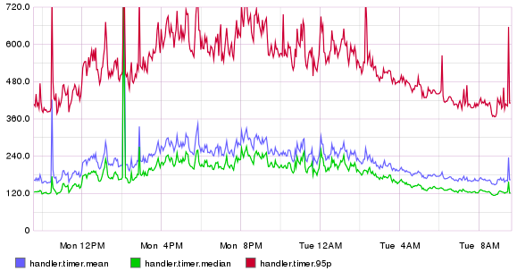
Here we increment a counter handler.requests each time we get a new incoming request. This can be then used to see how many requests per second the server is doing during a day. In addition we measure how long the total request took to process. Here’s an example what the results might look when the increasing load starts to slow the system and the latency starts to spike up. The blue (mean) and green (median) latencies are pretty tolerable, but the 95% starts to increase a lot, thus 5% of our users get a lot slower responses.

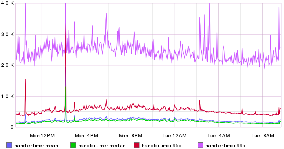
If we add the 99% percentile to the picture we see how bad the situation can really be:

Conclusion

Node.JS is not an optimal platform to do complex request processing where different requests might contain different amount of data, especially if we want to guarantee some kind of Service Level Agreement (SLA) that the service must be fast enough. A lot of care must be taken so that a single asynchronous callback can’t do processing for too long and it might be viable to explore other languages which are not completely single threaded.

Using HAProxy to do health checks to gRPC services

Haproxy is a great tool to do load balancing between microservers, but it current doesn’t support HTTP/2.0 nor gRPC directly. The only option now is to use tcp mode to load balance gRPC backend servers. It is however possible to implement intelligent health checks to gRPC enabled backends using “tcp-check send-binary” and “tcp-check expect binary” features. Here’s how:

First create a .proto service to represent a common way to obtain health check data from all of your servers. This should be shared with all your servers and projects as each gRPC endpoint can implement multiple different services. Here’s my servicestatus.proto as an example and it’s worth nothing that we should be able to add more fields into the StatusRequest and HealthCheckResult messages later if we want to extend the functionality without breaking the haproxy health check feature:

syntax = "proto3";

package servicestatus;

service HealthCheck {
  rpc Status (StatusRequest) returns (HealthCheckResult) {}
}

message StatusRequest {

}

message HealthCheckResult {
  string Status = 1;
}

The idea is that each service implements the servicestatus.HealthCheck service so that we can use same monitoring tools to monitor each and every different gRPC based service in our entire software ecosystem. In the HAProxy case I want that haproxy could call the HealthCheck.Status() function every few seconds and then the server would respond if everything is ok and that the server is capable of accepting new requests.  The server should set the HealthCheckResult.Status field to “MagicResponseCodeOK” string when everything is good so that we can look for the magic string in the response inside haproxy.

Then I extended the service_greeter example (in node.js in this case) to implement this:

var PROTO_PATH = __dirname + '/helloworld.proto';

var grpc = require('../../');
var hello_proto = grpc.load(PROTO_PATH).helloworld;

var servicestatus_proto = grpc.load(__dirname + "/servicestatus.proto").servicestatus;
function sayHello(call, callback) {
  callback(null, {message: 'Hello ' + call.request.name});
}

function statusRPC(call, callback) {
  console.log("statusRPC", call);
  callback(null, {Status: 'MagicResponseCodeOK'});
}

/**
 * Starts an RPC server that receives requests for the Greeter service at the
 * sample server port
 */
function main() {
  var server = new grpc.Server();
  server.addProtoService(hello_proto.Greeter.service, {sayHello: sayHello});
  server.addProtoService(servicestatus_proto.HealthCheck.service, { status: statusRPC });
  server.bind('0.0.0.0:50051', grpc.ServerCredentials.createInsecure());
  server.start();
}

main();

Then I also wrote a simple client to do a single RPC request to the HealthCheck.Status function:

var PROTO_PATH = __dirname + '/servicestatus.proto';

var grpc = require('../../');
var servicestatus_proto = grpc.load(PROTO_PATH).servicestatus;

function main() {
  var client = new servicestatus_proto.HealthCheck('localhost:50051', grpc.credentials.createInsecure());
  client.status({}, function(err, response) {
    console.log('Greeting:', response);
  });
}

main();

What followed was a brief and interesting exploration into how HTTP/2.0 protocol works and how gRPC uses HTTP/2.0 to work. After a brief moment with Wireshark I was able to explore the different frames inside a HTTP/2.0 request:

Screen Shot 2015-11-26 at 10.34.36

We can see here how the HTTP/2 request starts with first a Magic frame following with a SETTINGS frame. It seems that in this case we don’t need the  WINDOW_UPDATE frame when we later construct our own request. If we look closer on the packet #5 with Wireshark we can see this:

Screen Shot 2015-11-26 at 10.36.01

The Magic and SETTINGS are required in the start of each HTTP/2 request. After these gRPC sends a HEADERS frame which contains the interesting parts:

Screen Shot 2015-11-26 at 10.39.44

There’s also a DATA which in this case contains the protocolbuffers encoded payload of the function arguments. The DATA frame is analogous to the POST data payload in the HTTP/1 version, if that helps you to understand what’s going on.

What I did next is that I simply copied the Magic, SETTINGS, HEADERS and DATA frames as a raw Hex string and wrote a simple node.js program to test my work:

Screen Shot 2015-11-26 at 10.36.49

var net = require('net');

var client = new net.Socket();
client.connect(50051, '127.0.0.1', function() {
	console.log('Connected');

	var magic = new Buffer("505249202a20485454502f322e300d0a0d0a534d0d0a0d0a", "hex");
	client.write(magic);

	var settings = new Buffer("00001204000000000000020000000000030000000000040000ffff", "hex");
	client.write(settings);

	var headers = new Buffer("0000fb01040000000140073a736368656d65046874747040073a6d6574686f6404504f535440053a70617468212f736572766963657374617475732e4865616c7468436865636b2f537461747573400a3a617574686f726974790f6c6f63616c686f73743a3530303531400d677270632d656e636f64696e67086964656e746974794014677270632d6163636570742d656e636f64696e670c6465666c6174652c677a69704002746508747261696c657273400c636f6e74656e742d747970651061
	client.write(headers);

	var data = new Buffer("0000050001000000010000000000", "hex");
	client.write(data);

});

client.on('data', function(data) {
	console.log('Received: ' + data);
});

client.on('close', function() {
	console.log('Connection closed');
});

Now when I ran this node.js client code I correctly managed to create a gRPC request to the server and I could see the result, especially the MagicResponseCodeOK string. So how can we use this with HAProxy? We can simply define a backend with “mode tcp” and to concatenate the different HTTP/2 frames into one “tcp-check send-binary” blob and ask haproxy to look for the MagicResponseCodeOK string in the response. I’m not 100% sure yet that this works across all different gRPC implementations, but it’s a great start for a technology demonstration so that we don’t need to wait for HTTP/2 support in haproxy.

listen grpc-test
	mode tcp
	bind *:50051
	option tcp-check
	tcp-check send-binary 505249202a20485454502f322e300d0a0d0a534d0d0a0d0a00001204000000000000020000000000030000000000040000ffff0000fb01040000000140073a736368656d65046874747040073a6d6574686f6404504f535440053a70617468212f736572766963657374617475732e4865616c7468436865636b2f537461747573400a3a617574686f726974790f6c6f63616c686f73743a3530303531400d677270632d656e636f64696e67086964656e746974794014677270632d6163636570742d656e636f64696e670c6465666c6174652c677a69704002746508747261696c657273400c636f6e74656e742d74797065106170706c69636174696f6e2f67727063400a757365722d6167656e7426677270632d6e6f64652f302e31312e3120677270632d632f302e31322e302e3020286f73782900000500010000000100000000000000050001000000010000000000
	tcp-check expect binary 4d61676963526573706f6e7365436f64654f4b
	server 10.0.0.1 10.0.0.1:50051 check inter 2000 rise 2 fall 3 maxconn 100

There you go. =)

When Just IOPS Aren’t Enough – Optimal EBS Bandwidth Calculation

The current EBS features in Amazon EC2 environment offers really good performance and the marketing material and documentation boosts how different EBS types give IOPS, but a lesser talked thing is the bandwidth which EBS can offer. Traditional SATA attached magnetic hard disks can usually provide speeds from 40-150 MiB/s but really low amount of IOPS – something between 50-150 depending on rotation speed. With the Provisioned and GP2 EBS volume types it’s easy to focus on just getting enough IOPS but it’s important not to forget how much bandwidth the instance can get from the disks.

The EBS bandwidth in EC2 is limited by a few different factors:

  • The maximum bandwidth of the EBS block device
  • EC2 instance type
  • Is EBS-Optimised bit turned on for the instance

In most instance types the EBS traffic and the instance network traffic flows on the same physical NIC attached. In these cases the EBS-Optimised bit simply adds a QOS marker to the EBS packets. According to AWS documentation some instance types have a dedicated network interface for the EBS traffic and thus they don’t need to offer separated EBS-Optimised mode. This can be seen as the instances are natively always EBS-Optimised in the AWS documentation. It seems that the c4, d2 and m4 instance types seems to have this dedicated EBS NIC in the physical host.

The EBS type itself has bandwidth limitations. According to the documentation GP2 has maximum throughput of 160 MiB/s, Provisioned volume 320 MiB/s and magnetic 40-90 MiB/s. The GP2 and Provisioned bandwidth is determined on the volume size, so a small volume will not achieve the maximum bandwidth.

So to get maximum bandwidth in a single EC2 instance with EBS you should choose an instance type which is always EBS optimised, calculate maximum bandwidth of your EBS instance types and usually combine several EBS volumes together with stripped LVM to obtain best performance. For example a c4.4xlarge has max EBS bandwidth of 250 MiB/s and would require two GP2 EBS volumes (2 * 160 MiB/s) to max it out. According to my tests a single striped LVM logical volume which is backed up with two EBS volumes can achieve a constant read or write speed of 250 MiB/s while also transferring at 1.8 Gbps speed over the ethernet network to another machine.

Q&A on MongoDB backups on Amazon EC2

I just recently got this question from one of my readers and I just posted my response here for future reference:

I was impressed about your post about MongoDB because I have similar setup at my company and I was thinking maybe you could give me an advice.

We have production servers with mongodb 2.6 and replica set. /data /journal /log all separate EBS volumes. I wrote a script that taking snapshot of production secondary /data volume every night. The /data volume 600GB and it takes 8 hours to snapshot using aws snapshot tool. In the morning I restore that snapshot to QA environment mongodb and it takes 1 minute to create volume from snapshot and attach volume to qa instance. Now my boss saying that taking snapshot on running production mongodb drive might bring inconsistency and invalidity of data. I found on internet that db.fsynclock would solve the problem. But what is going to happen if apply fsynclock on secondary (replica set) for 8 hours no one knows.
We store all data (data+journal+logs) into the same EBS volume. That’s also what MongoDB documentation suggests: “To get a correct snapshot of a running mongod process, you must have journaling enabled and the journal must reside on the same logical volume as the other MongoDB data files.” (that doc is from 3.0 but it applies also to 2.x)
I suggest that you switch to having data+journal in the same EBS volume and after that you should be just fine with doing snapshots. The current GP2 SSD disks allows big volumes and great amount of IOPS so that you might be able to get away with having just one EBS volume instead of combining several volumes together with LVM. If you end up using LVM make sure that you use the LVM snapshot sequence which I described in my blog http://www.juhonkoti.net/2015/01/26/tips-and-caveats-for-running-mongodb-in-production
I also suggest that you do snapshots more often than just once per night. The EBS snapshot system stores only new modifications, so the more often you do snapshots, the faster each snapshot will be created. We do it once per hour.
Also after the EBS snapshot API call has been completed and the EBS snapshot process is started you can resume all your operations in the disk which was just snapshotted. In other words: The data is frozen at some atomic moment during the EBS snapshot API call. After that moment the snapshot will contain exactly that data what it was during that atomic moment. The snapshot progress just tells you when you can restore a new EBS volume from that snapshot and that your volume IO performance is degraded a bit because the snapshot is being copied to S3 behind the scenes.
If you want to use fsynclock (which btw should not be required if you use mongodb journal) then implement a following sequence and you are fine:
  1. fsynclock
  2. XFS freeze (xfs_freeze -t /mount/point)
  3. EBS snapshot
  4. XFS unfreeze
  5. fsyncUnlock (xfs_freeze -u /mount/point)
The entire process should not take more than a dozen or so seconds.


Windows script to convert video into jpeg sequence

I do a lot of Linux scripting but Windows .BAT files are something which I haven’t touched since the old MS DOS times.

Here’s a simple .BAT file which you can use to easily convert video into a jpeg sequence using ffmpeg:

echo Converting %1 to jpeg sequence
mkdir "%~d1%~p1%~n1"
c:\work\ffmpeg\bin\ffmpeg.exe -i %1 -q:v 1 %~d1%~p1%~n1\%~n1-%%05d.jpg

You can copy this into “%userdata%\SendTo” so that you can use this by selecting a file and right clicking. It creates a sub directory into the source file directory and writes the sequence there.
Most of the magic is in the weird %~d1 variables which I found out from this StackExchange. I use this to convert my GoPro footage into more suitable jpeg sequence which I then use with DaVinci Resolve.

DNA Welho cable modem IPv6 with Ubiquiti EdgeMax

DNA/Welho recently announced their full IPv6 support. Each customer gets an /56 prefix via dhcpv6. Here’s my simple configuration on how to get things running with EdgeMax. This assumes that the cable modem is in bridged mode and connected to eth0. eth1 is the LAN port.

set firewall ipv6-name WANv6_IN default-action drop
set firewall ipv6-name WANv6_IN description 'WAN inbound traffic forwarded to LAN'
set firewall ipv6-name WANv6_IN enable-default-log
set firewall ipv6-name WANv6_IN rule 10 action accept
set firewall ipv6-name WANv6_IN rule 10 description 'Allow established/related sessions'
set firewall ipv6-name WANv6_IN rule 10 state established enable
set firewall ipv6-name WANv6_IN rule 10 state related enable
set firewall ipv6-name WANv6_IN rule 15 action accept
set firewall ipv6-name WANv6_IN rule 15 description 'Allow ICMPv6'
set firewall ipv6-name WANv6_IN rule 15 protocol ipv6-icmp
set firewall ipv6-name WANv6_IN rule 20 action drop
set firewall ipv6-name WANv6_IN rule 20 description 'Drop invalid state'
set firewall ipv6-name WANv6_IN rule 20 state invalid enable
set firewall ipv6-name WANv6_LOCAL default-action drop
set firewall ipv6-name WANv6_LOCAL description 'Internet to router'
set firewall ipv6-name WANv6_LOCAL enable-default-log
set firewall ipv6-name WANv6_LOCAL rule 1 action accept
set firewall ipv6-name WANv6_LOCAL rule 1 description 'allow established/related'
set firewall ipv6-name WANv6_LOCAL rule 1 log disable
set firewall ipv6-name WANv6_LOCAL rule 1 state established enable
set firewall ipv6-name WANv6_LOCAL rule 1 state related enable
set firewall ipv6-name WANv6_LOCAL rule 3 action accept
set firewall ipv6-name WANv6_LOCAL rule 3 description 'allow icmpv6'
set firewall ipv6-name WANv6_LOCAL rule 3 log disable
set firewall ipv6-name WANv6_LOCAL rule 3 protocol icmpv6
set firewall ipv6-name WANv6_LOCAL rule 5 action drop
set firewall ipv6-name WANv6_LOCAL rule 5 description 'drop invalid'
set firewall ipv6-name WANv6_LOCAL rule 5 log enable
set firewall ipv6-name WANv6_LOCAL rule 5 state invalid enable
set firewall ipv6-name WANv6_LOCAL rule 8 action accept
set firewall ipv6-name WANv6_LOCAL rule 8 description 'DHCPv6 client'
set firewall ipv6-name WANv6_LOCAL rule 8 destination port 546
set firewall ipv6-name WANv6_LOCAL rule 8 log disable
set firewall ipv6-name WANv6_LOCAL rule 8 protocol udp
set firewall ipv6-receive-redirects disable
set firewall ipv6-src-route disable
set interfaces ethernet eth0 address dhcp
set interfaces ethernet eth0 description wan
set interfaces ethernet eth0 dhcpv6-pd pd 0 interface eth1 host-address '::1'
set interfaces ethernet eth0 dhcpv6-pd pd 0 interface eth1 service slaac
set interfaces ethernet eth0 dhcpv6-pd pd 0 prefix-length 56
set interfaces ethernet eth0 dhcpv6-pd rapid-commit enable
set interfaces ethernet eth0 firewall in ipv6-name WANv6_IN
set interfaces ethernet eth0 firewall local ipv6-name WANv6_LOCAL
set interfaces ethernet eth0 ipv6 dup-addr-detect-transmits 1

Here’s a quick explanation on the key details: dhcpv6-pd is a way to ask for a prefix block from the ISP. The ISP will assign a /128 point-to-point ip to the WAN interface which the ISP uses as the gateway to the prefix which it gives to you. You could simply just say “set interfaces ethernet eth0 dhcpv6-pd” and you would only get the /128 point-to-point link, which is enough for the router to connect to public ipv6 but not else.

The “set interfaces ethernet eth0 dhcpv6-pd pd 0” block is the request for the /56 prefix. This prefix will be then assigned to one interface (eth1) so that the interface will get an ip ending with ::1 and then the subnet is served via a slaac protocol to the clients.

Notice that there seems to be a small bug: If you did just “set interfaces ethernet eth0 dhcpv6-pd” and committed that, additional “dhcpv6-pd pd” settings wont work unless you first “delete interfaces ethernet eth0 dhcpv6-pd” and commit that.

IPv6 changes several key features when compared to IPv4 so be ready to learn again how ARP requests works (hint, there’s no ARP requests any more), how multicast is used in many places and how interfaces have several IPv6 addresses in several networks (link-local, public etc). Here’s one helpful page which explains more on the prefix delegation.

Continuous Integration pipeline with Docker

I’ll describe our Continuous Integration pipeline which is used by several teams to develop software which is later deployed as Docker Containers. Our programmers use git to develop new features into feature branches which are then usually merged into master branch. The master branch represents the current development of the software. Most projects also have a production branch which always contains code which is ready to be deployed into production at any given moment. Some software packages use version release model so each major version has its own branch.

As developers develop their code they always run at least unit tests locally in their development machine. New code is committed into feature branch, which is merged by another developer into master and pushed to the git repository. This triggers a build in a Jenkins server. We have several Jenkins environments, the most important are testing and staging. Testing provides a CI environment for the developers to verify that their code is production compatible and the staging is for the testing team so that they can have their time to test a release candidate before its actually deployed into production.

High level anatomy of a CI server

The CI service runs a Linux with Docker support. A Jenkins instance is currently installed directly into the host system instead of a container (we had some issues with it as it needs to launch containers). Two sets of backend services are also started into the server: A minimal set required for a development environment. These containers run with –net=host mode and they bind to their default ports. These are used for the unit tests.

Then there’s a separated set of services inside containers which form a complete set that looks just like production environment. The services also obtain fresh backups from production databases so that the developers can test the new code against a copy of live data. These services run with the traditional docker mode, so they each have their own IP from the 178.18.x.x address space. More on this later.

ci-build2

Services for development environment and when running unit tests

Developers can run a subset of required services in their development laptops. This means that for each database type (redis, mongodb etc) only a minimal amount of processes are started (say one mongodb, one redis and no more). This is so that the environment doesn’t consume too much resources. The tests can also be programmed to assume that there’s actual databases behind. When the tests are executed in a CI machine a similar set of services is found on the ports at localhost of the machine. So the CI machine has both a set of services bound to localhost default ports and then a separated set of services which represent the production environment (see next paragraph)

We also use a single Vagrant image which contains this minimal set of backend services inside containers so that the developers can easily spawn the development environment into their laptops.

Build sequence

When a build is triggered the following sequence is executed. A failure in any step break the execution chain and the build is marked as a failure:

  1. Code is pulled from the git repository.
  2. The code includes a Dockerfile which is then used to build a container which is tagged with the git revision id. This results that each commit id has one and exactly one container.
  3. The container is started so that it executes the unit test suite inside the container. This accesses a set of empty databases which are reserved for unit and integration testing.
  4. Integration test suite is executed: This means that first a special network container is started with “–name=”networkholder” which acts as a base for the container network and it runs redir which is used to redirect certain ports from inside the container to the host system so that some depended services (like redis, mongodb etc) can be accessed as they would be in the container “localhost”. Then the application container is started with the –net=”container:networkholder” so that it reuses the network container network stack and it starts the application so that it listens for incoming requests. Then a third container is started into the same network space (–net=”container:networkholder) and this executes the integration test suite.
  5. A new application container (which usually replaces an existing container from the previous build) so that the developers can access the running service across the network. This application container has access to production like set of backend services (like databases) which contains a fresh copy of the production data.
  6. A set of live tests are executed against the application container launched in previous step. These tests are programmed to assume that they can be executed continuously in the production. This step verifies that the build can work with a similar deployment what the production has.
  7. The build is now considered to be successful. If this was a staging build then the container is uploaded to a private Docker registry so that it could be deployed into production. Some services run an additional container build so that all build tools and other unnecessary binaries are stripped from the container for security reasons.

Service naming in testing, staging and production

Each of our service has an unique service name, for example a set of mongodb services would have names “mongodb-cluster-a-node-1” to “mongodb-cluster-a-node-3”. This name is used to create a dns record: “mongodb-cluster-a-node-1.us-east-1.domain.com” so that each production region has its own domain (here “us-east-1.domain.com”). All our services use /etc/resolv.conf to add the region domain into its search path. This results that the applications can use the plain service name without the domain to find the services. This has the additional benefit that we can run the same backend services in our CI servers so that the server has a local dns resolver which resolves the host names to docker container.

Consider this setup:

  • Application config has setting like mongodb.host = “mongodb-cluster-a-node-1:27017”
  • Production environment the service mongodb-cluster-a-node-1 is deployed into some arbitrary machine and a DNS record is created: mongodb-cluster-a-node-1.us-east-1.domain.com A 10.2.2.1
  • Testing and Staging environments both run mongodb-cluster-a-node-1 service locally inside one container. This container has its own IP address, for example 172.18.2.1.

When the application is run in testing or staging: Application resolves mongodb-cluster-a-node-1. The request goes to a local dnsmasq in the CI machine, which resolves the name “mongodb-cluster-a-node-1” into a container at ip 172.18.2.1. Application connects to this ip which is locally in the same machine.

When the application is run in production: Application resolves mongodb-cluster-a-node-1. The request goes into the libc dns lookup code which uses the search property from /etc/resolv.conf. This results that a DNS query is eventually done for mongodb-cluster-a-node-1.us-east-1.domain.com, which returns an IP in an arbitrary machine.

This setup allows us to use the same configurations in both testing, staging and production environments, so that we can verify that all high availability client libraries can connect to all required backends and that the software will work in the production environment.

Conclusion

This setup suits our needs quite well. It leverages the sandboxing which Dockers gives us and enables us to do new deployments with great speed: The CI server needs around three minutes to finish a single build plus two minutes for deployment with our Orbitctl tool, which deserves its own blog post. The developers can use the same containers in a compact Vagrant environment which we use to run our actual production instances, reducing the overhead for maintaining separated environments.

Comparing Kubernetes with Orbit Control

I’ve been programming Orbit Control as a tool to deploy Docker containers for around half a year which we have been running in production without any issues. Recently (Nov 2014) Google released Kubernetes, its cluster container manager, which slipped under my radar until now. Kubernetes seem to contain several nice design features which I had already adopted into Orbitctl, so it looks like a nice product after a quick glance. Here’s a quick summary on the differences and similarities between Kubernetes and Orbitctl.

  • Both use etcd to store central state.
  • Both deploy agents which use the central state from etcd to converge the machine into the desired state.
  • Kubernetes relies on SaltStack for bootstrapping the machines. Currently we use Chef to bootstrap our machines but for Orbitctl it’s just one static binary which needs to be shipped into the machine, so no big difference here.
  • Orbitctl has just “services” without any deeper grouping. Kubernetes adds to this by defining that a Service is a set of Pods. Each pod contains containers which must be running in the same machine.
  • Orbit doesn’t provice any mechanisms for networking. The containers within a Kubernetes Pod share a single network entity (ie. and IP address) and the IP address is routable and accessible between machines running the pods. This seems to help preventing port conflicts in a Kubernetes deployment.
  • Orbit provides a direct access for Docker api which doesn’t hide anything where Kubernetes encapsulates several Docker details (like networking, volume mounts etc) into its own manifest format.
  • Orbitctl has “tags”, Kubernetes has “labels” which have more use cases within Kubernetes than what Orbit currently has for its tags.
  • Orbitctl relies on operators to specify which machines (according to tag) run which service. Kubernetes has some kind of automatic scheduler which can take cpu and memory requirements in account when it distributes the pods.
  • Both use json to define services with pretty similar syntax which is then loaded using a command line tool into etcd.
  • Orbitctl can automatically configure haproxies to specific set of services within a deployment. Kubernetes has similar software router, but it can’t support haproxy yet. There’s open issues on this, so it is coming in the future.
  • Kubernetes has several networking enchantments coming up later in their own feature roadmap. Read more here.
  • Both have support for health checks.
  • Orbit supports deployments across multiple availability zones but not across multiple regions. Kubernetes says it’s not supposed to be distributed across availability zones, probably because its lacking some HA features as it has a central server.

Kubernetes looks really promising, at least when they reach 1.0 version which has nice planned list of features. Currently its lacking some critical features like haproxy configuration, support for deployments across availability zones so it’s not production ready for us, but it’s definitively something to keep an eye on.

Tips and caveats for running MongoDB in production

A friend of mine recently asked about tips and caveats when he was planning a production MongoDB installation. It’s a really nice database for many use cases, but it, as every other, has its quirks. As we have been running MongoDB for several years we have encountered quite many bugs and issues with it. Most of them have been fixed during the years, but some are still persisting. Here’s my take on few good to know keypoints:

Slave with replication lag can get slaveOk=true queries

MongoDB replication is asynchronous. The master stores every operation into an oplog which the slaves read one operation at a time and apply the commands into their own data. If a slave can’t keep up it will be delayed and thus it won’t contain all the updates which the master has already seen. If you are running a software which is doing queries with slaveOk=true then mongos and some of the client drivers can direct those queries into one of the slaves. Now if your slave is lagging behind with its replication then there’s a very good change that your application can get older data and thus might end up corrupting your data set logically. A ticket has been acknowledged but not scheduled for implementation: 3346.

There’s two options: You can dynamically check the replication lag in your application and program your application to drop the slaveOk=true property in this case, or you can reconfigure your cluster and hide the lagging slave so that mongos will not drive slaveOk queries to it. This brings us to the second problem:

Reconfiguring cluster often causes it to drop primary database for 10-15 seconds.

There’s really no other way saying this, but this sucks. There are number of operations which still, after all these years, causes the MongoDB cluster to throw its hands into the air, drop primary from the cluster and completely rethink who should be the new master – usually ending up keeping the exact same master than it was before. There have been numerous Jira issues to this but they’re half closed as duplicate and half resolved: 6572, 5788, 7833 plus more.

Keep your oplog big enough, but cluster size small enough.

If your database is getting thousands of updates per second the time what the oplog can hold will start to shrink. If your database is also getting bigger then some operations might take too long that they no longer can complete during the oplog time window. Repairs, relaunches and backup restores are the main problems. We had one database which had 100GB oplog which could hold just about 14 hours of operations – not even closely enough to keep the ops guys sleep well. Another problem is that in some cases the oplog will mostly live in active memory, which will cause penalties to the overall database performance as the hot cacheable data set shrinks.

Solutions? Either manually partition your tables into several distinct mongodb clusters or start using sharding.

A word on backups

This is not a MongoDB related issue, backups can be hard to implement. After a few tries here’s our way which has served us really well: We use AWS so we’re big fans of the provisioned IOPS volumes. We mount several EBS volumes into the machine as we want to keep each volume less than 300GB if possible, so that AWS EBS snapshots wont take forever. We then use LVM with striping to combine the EBS volumes into one LVM Volume Group. On top of that we create a Logical Volume which spans 80% of the available space and we create an XFS filesystem on it. The remaining 20% is left for both backups and emergency space if we need to quickly enlarge the volume. XFS allows growing the filesystem without unmounting it, right on a live production system.

A snapshot is then done with the following sequence:

  1. Create new LVM snapshot. Internally this does XFS lock and fsync, ensuring that the filesystem has fully synchronous status. This causes MongoDB to freeze for around four seconds.
  2. Create EBS snapshots for each underlying EBS volumes. We tag each volume with timestamp, position in the stripe, stripe id and “lineage” which we use to identify the data living in the volume set.
  3. Remove the LVM snapshot. The EBS volume performance is now degraded until the snapshots are completed. This is one of the reason why we want to keep each EBS volume small enough. We usually have 2-4 EBS volumes per LVM group.

Restore is done in reverse order:

  1. Use AWS api to find the most recent set of EBS volumes for given lineage which contains all EBS volumes and which snapshots have been successfully completed.
  2. Create new EBS volumes from the snapshots and mount the volumes into the machine.
  3. Spin up the LVM so that kernel finds the new volumes. The LVM will contain the actual filesystem Logical Volume and the snapshot. The filesystem volume is corrupted and cannot be used per-se.
  4. Restore the snapshot into the volume. The snapshot will contain the fixed state which we want to use, so we need to merge it into the volume where the snapshot was taken from.
  5. The volume is now ready to use. Remove the snapshot.
  6. Start MongoDB. It will replay the journal and then start reading the oplog from the master so that it can get up to date with the rest of the cluster. Because the volumes were created from snapshots the new disks will be slow for at least an hour, so don’t be afraid that mongostat says that the new slave isn’t doing anything. It will, eventually.

Watch out for orphan Map-Reduce operations

If a client doing map-reduce gets killed the map-reduce operation might stick and keep using resources. You can kill them but even the kill operation can take some time. Just keep an eye out for these.

Great Chinese Firewall DDOSing websites

We recently got reports from two different small eCommerce related websites who started to see big amounts of traffic originating from Chinese IP addresses which contained the same path as our SDK which is shipped within mobile games, but destined into their ip address.

This made no sense at all.

We of course responded to the hostmasters tickets and assured that we would do everything to find the reason what is causing this, because effectively it looked like we were sending a distributed denial service attack against these websites.

After some googling we found out first this post: http://comments.gmane.org/gmane.network.dns.operations/4761 and then this better blog which described exactly what we had seen. https://en.greatfire.org/blog/2015/jan/gfw-upgrade-fail-visitors-blocked-sites-redirected-porn

So what’s going on is that if an url is blocked by the Chinese firewall the firewall DNS will respond with another ip which goes into another working website instead of the ip where it should go. According to the blog post the motivation might be that China wants the users to think that everything is working by sending them to another webpage. Too bad that it ends up causing a lot of harm into innocent admins all around the world.

Currently we are looking to change our systems to direct the Chinese users into another CDN host which aren’t affected, but as the previous Chinese firewall problem was just a couple of months ago I don’t see any way to easily fix this issue for good.

Raspberry Pi as a 3G to WiFi access point and home automation

I’ve just deployed a Raspberry Pi into our summer cottage to function as a general purpose home automation and internet access point. This allows visitors to connect to internet via wifi and also enables remote administration, environmental statistics and intrusion alerts.

Parts:

  • Raspberry Pi, 4GB memory card
  • PiFace Digital (for motion sensors and heating connection, not yet installed)
  • D-Link DWA-127 Wi-Fi USB (works as an access point in our case)
  • Huawei 3G USB dongle (from Sonera, idVendor: 0x12d1 and idProduct:          0x1436) with a small external antenna.
  • Two USB hubs, one passive and another active with 2A power supply
  • Old TFT display, HDMI cable and keyboard

I’m not going into the details how to configure this, but I’ll give a quick summary:

  • Sakis3G script to connect the 3G to Internet. Works flawlessly.
  • umtskeeper script which makes sure that sakis3g works always. Can reset USB bus etc. Run from /etc/rc.local on startup.
  • hostapd to make the D-Link WiFi to act as an access point.

In addition I run OpenVPN to connect the network into the rest of my private network, so I can always access the rpi remotely from anywhere. This also allows remote monitoring via Zabbix.

Plans for future usage:

  • Connect to the building heating system for remote administration and monitoring.
  • Attach USB webcams to work as CCTV
  • Attach motion sensors for security alarm. Also record images when sensors spot motion and upload directly to internet.
  • Attach a big battery so that the system will be operational during an extended power outage.

Quick way to analyze MongoDB frequent queries with tcpdump

MongoDB has an internal profiler, but it’s often too complex for a quick statistics to see what kind of queries the database is getting. Luckily there’s an easy way to get some quick statistics with tcpdump. Granted, these examples are pretty naive in terms of accuracy, but they are really fast to do and they do give out a lot of useful information.

Get top collections which are getting queries:

tcpdump dst port 27017 -A -s 1400 |grep query | perl -ne '/^.{28}([^.]+\.[^.]+)(.+)/; print "$1\n";' > /tmp/queries.txt
sort /tmp/queries.txt | uniq -c | sort -n -k 1 | tail

The first command will dump the beginning of each packet as string which goes into MongoDB and it will then filter out everything except queries. The perl regexp clause will pick the target collection name and print it to stdout. You should run this around 10 seconds and then stop it with Ctrl+C. The next command sorts this log and prints top collections to stdout. You can run these commands both in your MongoDB machine or in your frontend machine.

You can also get more detailed statistics about the query by looking at the tcpdump. For example you can spot keywords like $and, $or, $readPreference etc which can help you to determine what kind of queries there are. Then you can pick up the queries you might want to cache with memcached or redis, or maybe to move some queries to the secondary instances.

Check out also this nice tool called MongoMem, which can tell you how much each of your collections are stored in the physical memory (RRS). This is also known as the “hot data”.

How to establish and run a techops team

As a company grows, there comes a point when it’s no longer feasible that the founders and programming gurus keep maintaining the servers. Your clients are calling in the middle of the weekend just to tell that a server is down and you didn’t even notice. Sounds familiar? It’s time you spin up the TechOps team.

TechOps stands for Technical Operations. It’s very closely related to a Dev Ops team (Development Operations) and in some organizations those are same. TechOps task is to maintain your fleet of servers, mostly importantly your production servers and to make sure that your production is working by monitoring constantly its performance, both hardware and software. This is extended some what from the traditional sysadmin task, because a TechOps team is primarily responsible for the production environment. If it also needs to get its hands dirty on maintaining servers, then so be it, but the ideology is that those are your valuable guys who make sure that everything is working as they should.

In a small company it’s usually not required to have dedicated guys on the TechOps team. In our company, for example, we have one dedicated guy and two additional guys, who share the TechOps duties. The two guys are actually software designers of the two different products our company runs, which has been a great benefit. This way the TechOps team has always direct knowledge of all the products we are supposed to be operating. The one full time TechOps guy writes automation scripts, monitoring scripts and does most of the small day-to-day operations.

Knowing how your production runs

TechOps should know everything what’s happening in the production servers. This means that they should be capable of understanding how the products actually work, at least in some detail. They can also be your DBA’s (Database Administrator), taking a close look on actual database operations and talking constantly with the programmers who design the applications database layers.

TechOps should manage how new builds of the software is distributed and deployed on the production servers and they should be the only guys who have actually the need to log into the production boxes. You don’t give your developers access to the production servers, because they might not know how the delicate TechOps automation scripts are working on those boxes, so you don’t want any outsiders to mess the systems up.

Monitoring your production

Monitoring is a key part of TechOps. You should always have some kind of monitoring software running, which gathers data from your servers, applications and networks, displays them in an easy and human readable way and triggers warnings and alerts if something unexpected happens. Most common tools for this job is Nagios and Zabbix, which I prefer. They should also store metrics from the past, allowing operators to look for odd patterns and to help with root cause analysis.

What ever your monitoring solution is, you need to maintain it constantly.  You can’t let old triggers and items to lay in a degraded state. If you remove a software or a server, you need to remove those items also from your monitoring software. When you add something new to your production environment, it’s the TechOps guys who will also think how the new piece is monitored and to setup this monitoring. They also need to watch the new component for a while so they can adjust alerts for the different meters (zabbix calls these “items”), so an appropriate alert is escalated when needed.

TechOps also usually take shifts to be on standby in case there’s problems in the production. This is mostly combined with the monitoring solution, which will send alerts in form of emails, SMS messages and push notifications into the phone of the on-duty TechOps engineer. Because of this, you need to design proper escalation procedures for your environment:

For an example, our company tracks about 7800 zabbix items from around 100 hosts. We also run Graphite to get analytics from inside our production software, which tracks additional  2800 values.

Design and implement meaningful alerts to your environment

Zabbix divides the alerts into following severities: Information, Warning, Average, High and Disaster. You should plan your alerts so that they will trigger an alert with appropriate severity. We have found the following rule-of-thumb to be an excellent way on this:

  • Information: Indicates some anomaly which is not dangerous but should be noted.
  • Warning: Indicates a warning condition within system, but does not affect production in any way.
  • Average: Action needed during working hours. Does not affect production but the system is in degraded state and needs maintenance. You can go for a lunch before taking action on this.
  • High: Immediate action needed during working hours and during alert service duty. Production systems affected.
  • Disaster: Immediate action needed around the clock. Money is leaking, production is not working. All is lost.

For example if you have three web frontend servers in a high-availability configuration behind load balancer and one of those servers goes down. This should not affect your production, but you have enough performance that the two remaining servers can handle it just fine, so this is an average problem. If another server goes down, this most likely will affect your production performance and you don’t have any servers to spare, this is a high problem. It’s a disaster if all your servers go down.

Do not accept single point of failures

TechOps should require that all parts of production environment should be robust enough to handle failures. Anything can break, so you must have redundancy designed into your architecture from ground up. You simply should not accept a solution which can’t be clustered for high availability. TechOps must be in constant discussion with the software developers to determine how a certain piece of software can be deployed safely into the production environment.

TechOps should log each incident somewhere, so you can use it later to spot trends and to determine if some frequently occurring problem can be fixed permanently. This also doubles as an audit log for paying the on-duty TechOps engineers appropriate compensation because he woke up at 4 AM at night to fix your money making machine.

Automate as much as you can

Modern tools, specially having your infrastructure in the cloud, allows you to automate a great deal of day-to-day operation tasks. Replacing a failed database instance should be just two clicks away (one for the action and another for confirmation). Remember, you can use scripts to do everything what a human operator does! It’s not always cost efficient to write scripts for everything, but after you do the same thing for the 3rd time, you know that you should be writing a script for it instead of doing it yet again manually.

Chef and Puppet are examples of great pieces of automation software which will help you to manage your servers and the software running inside. They both have a steep learning curve, but it’s well worth it.

Conclusions

Running TechOps is a never-ending learning process. Starting one is hard, but as the team progresses the day-to-day operations become increasingly more efficient and you are rewarded with increasingly better production with higher uptime. It also helps your helpdesk operations because you clients won’t see your servers being down. This ultimately will result with a good ROI, because you will have less downtime with faster reaction times when things to wrong.

Avointa maastotietodataa – löytyisikö sitä uutta kiipeiltävää?

Osana valtionhallinnon avoimen datan hanketta Maanmittauslaitos avasi vihdoin arkistonsa kaiken kansan nähtäville. Ehkä mielenkiintoisin näistä on Maastotietokanta, joka sisältää eritellysti yhtenä valtavana tietokantana kaikki Maanmittauslaitoksen kartoittamat yksityiskohdat maastosta. Kiipeilijät ovat pitkään etsineet uusia potentiaalisia kiipeilypaikkoja selailemalla karttoja, mutta voisiko hommaa helpottaa?

Maanmittauslaitos määrittelee Kiven seuraavasti:

Yli 2.5 m korkea tai yleisesti tunnettu tai vähäkivisellä seudulla selvästi ympäristöstään erottuva kivilohkare. Alueella, jossa on runsaasti yli 2.5 m korkeita kivilohkareita, vain selvimmin ympäristöstään erottuvat kivilohkareet tallennetaan.

Omaan korvaani tuo kuulostaa melko hyvältä potentiaalisen boulderin määritelmältä! Analysoin koeluontoisesti kaikki Suomesta löytyvät 483713 kiveä ja jaoin ne kartalla noin 1000 * 500 metrin lohkoihin. Tämän jälkeen piirsin kaikki eniten kiviä sisältäneet lohkot Google Mapsin päälle. Tästä kartasta voi klikata yksittäistä pistettä, jolloin pääsee katsomaan maastokarttaa kyseisestä kohdasta.

Tämä analyysi ei tietenkään löydä boulderointiin sopivia kiviä suoraan, vaan se toimii lähinnä apuna ohjaamaan etsintää suoraan mahdollisesti potentiaalisille alueille. Jos alue näyttää kiinnostavalta, niin sitten vaan GPS:n kanssa keväiseen luontoon! Huomioithan kuitenkin access-asiat! Tämä on vasta yksi esimerkki miten aineistoa voi käyttää kiipeilyn hyväksi. Moni varmasti keksii parempia tapoja!

Siirry yleiskarttaan tästä.

Kuva: Juha Immonen

Teknisesti orjentoituneet voivat katsoa lähinnä omaan käyttöön tehdyt lähdekoodit GitHubista. Itse aineiston kopioin kätevästi Kapsi Ry:n palvelimelta.

Setting backup solution for my entire digital legacy (part 2 of 2)

As part of my LifeArchive project, I had to verify that I have sufficient methods to back all my valuable assets so well that they will last for decades. Sadly, there isn’t currently any mass media storage available that is known to function for such a long time, and in any way you must prepare for losing a site due to floods, fire and other disasters. This post explains how I solved my backup needs for my entire digital legacy. Be sure to read the first part: LifeArchive – store all your digital assets safely (part 1 of 2)

The cheapest way to store data currently is to use hard disks. Google, Facebook, The Internet Archive, Dropbox etc are all known to host big data centers with a lot of machine with a lot of disks. Also at least Google is known to use tapes for additional backups, but they are way too expensive for this kind of small usage.

Disks have also their own problem. The biggest problem is that they tend to break. Another problem is that they might corrupt your data, which is a problem with traditional raid systems. As I’m a big fan of ZFS, my choose was to build a SAN on top of it. You can read more on this process from this blog post: Cheap NAS with ZFS in HP MicroServer N40L

Backups

As keeping your eggs in one basked is just stupid, having a good and redundant backup solution is the key to success. As in my previous post, I concluded that using cloud providers to solely host your data isn’t wise, but they are a viable choice for doing backups. I’ve chosen to use CrashPlan, which is a really nice cloud based software for doing increment backups. Here are the cons and the pros for CrashPlan:

Pros:

  • Nice GUI for both backing up and restoring files
  • Robust. The backups will eventually complete and the service will notify you by email if something is broken
  • Supports Windows, OS X, Linux and Solaris / OpenIndiana
  • Infinitive storage on some of the plans
  • Does increment backups, so you can find the lost file from history.
  • Allows you to backup to both CrashPlan cloud and to your own storage if you run the client in multiple machines.
  • Allows you to backup to your friends machine (this doesn’t even cost you anything), so you can establish a backup ring with a few of your friends.

Cons:

  • It’s still a black-box service, which might break down when you least expect
  • CrashPlan cloud is not very fast: Upload rate to CrashPlan cloud is around 1Mbps and download (restore) around 5Mbps
  • You have to fully trust and rely on the CrashPlan client to work – there’s no another way to access the archive except using the client.

I setup the CrashPlan client to backup into its cloud and in addition to Kapsi Ry’s server where I’m running a copy of the CrashPlan client. Running your own client is easy and it gives me a much faster way to recover the data when I need to. As the data is encrypted, I don’t need to worry that there’s also a few thousand other users in the same server.

Another parallel backup solution

Even when CrashPlan feels like a really good service, I still didn’t want to trust solely to its services. I can always somehow forget to enter my new credit card number and let the data there expire, only to have a simultaneous fatal accident on my NAS. So that’s why I wanted to have a redundant backup method. I happen to get another used HP MicrosServer for a good bargain, so I setup it similarly to have three 1TB disks which I also happend to have laying around unused from my previous old NAS. Used gear, used disks, but they’re good enough to act as my secondary backup method. I will of course still receiver email notifications on disk failures and broken backups, so I’m well within my planning safety limits.

This secondary NAS lives at another site and it’s connected with an openvpn network to the primary server in my home. It also doesn’t allow any incoming connections from anywhere outside, so it’s also quite safe. I setup a simple rsync script from my main NAS to sync all data to this secondary NAS. The rsync script uses –delete -option, so it will remove files which have been deleted from the primary NAS. Because of this I also use a crontab entry to snapshot the backup each night. This will protect me if I accidentally delete files from the main archive. I keep a week worth of daily snapshots and a few month of weekly snapshots.

One best pros with this when comparing to CrashPlan is that the files are sitting directly on your filesystem. There’s no encryption nor any proprietary client and tools you need to rely, so you can safely assume that you can always get an access to your files.

There’s also another option: Get a few USB disks and setup a schema where you automatically copy your entire archive to one disk. Then every once in a while unplug one of those, put it somewhere safe and replace it with another. I might do something like this once a year.

Verifying backups and monitoring

“You don’t have backups unless you have proven you can restore from them.” – a well known truth that many people tend to forget. Rsync backups are easy to verify, just run the entire archive thru sha1sum on both sides and verify that the checksums match. CrashPlan is a different beast, because you need to restore the entire archive to another place and verify it from there. It’s doable, but currently it can’t be automated.

Monitoring is another thing. I’ve built all my scripts so that they will email me if there’s a problem, so I can react immediately on error. I’m planning to setup a Zabbix instance to keep track, but I haven’t yet bothered.

Conclusions

Currently most of our digital assets aren’t stored safely enough that you can count that they all will be available in the future. With this setup I’m confident that I can keep all my digital legacy safe from hardware failures, cracking and human mistakes. I admit that the overal solution isn’t simple, but it’s very well doable for an IT-savvy person. The problem is that currently you can’t buy this kind of setup anywhere as a service, because you can’t be 100% sure that the service will keep up in the upcoming decades.

This setup will also work as a personal cloud, assuming that your internet link is fast enough. With the VPN connections, I can also let my family members to connect into this archive and let them store their valuable data. This is very handy, because that way I will know that I can access my parents digital legacy, who probably can’t do all this by themselves alone.